library(tidyverse) # Pipeline of works
library(dplyr) # Data wrangling
library(ggplot2) # Data visualization
library(GGally) # Scatterplot matrix in the framework of ggplot
library(ggpubr) # Arranging ggplot objects in rows and columns
library(factoextra) # Visualization of resultsPrincipal Component Analysis
Problem Statement
- Suppose that \(\mathbf{x}_i=\{x_{i1},x_{2i},\ldots,x_{ip}\}\in\mathbb{R}^{p}; i=1,2,\ldots,n\) is our observed data.
- Let \(X_1,X_2,\ldots,X_p\) be the \(p\) feature vectors and serve as the columne of \(X\in\mathbb{R}^{n\times p}\)
- Let us assume that \(\mathbf{x}_i\) is centered that is it has \(\mathbf{0}\) mean, however, \(\text{cov}(\mathbf{x}_i)=\Sigma\).
Objective of PCA
- Principal component analysis (PCA) yields a low-dimensional representation of \(X\) with maximal variability.
- The idea of PCA is that not all dimension of \(\mathbb{R}^p\) where \(\mathbf{x}_i\)’s are belong to are important. Rather, there is a small number of orthongonal dimensions that can account maximum variation in \(X\).
- PCA seeks \(Y_1,Y_2,\ldots,Y_r\), where \(r<p\), that are independent linear combinations of \(X_1,X_2,\ldots,X_p\) so that maximum variation in \(X\) can be explained such that \(V(Y_1)\ge V(Y_2)\ge\ldots\ge V(Y_r)\). Mathematically, \[\begin{align*} Y_1&=X\mathbf{a}_1=a_{11}X_1+a_{12}X_2+\ldots+a_{1p}X_p\\ Y_2&=X\mathbf{a}_2=a_{21}X_1+a_{22}X_2+\ldots+a_{2p}X_p\\ &\vdots\\ Y_r&=X\mathbf{a}_r=a_{r1}X_1+a_{r2}X_2+\ldots+a_{rp}X_p\\ \end{align*}\] therefore, we have \[\begin{align*} \text{var}(Y_i)=\mathbf{a}_i^T\Sigma\mathbf{a}_i\quad\text{ and }\quad \text{cov}(Y_i,Y_j)=\mathbf{a}_i^T\Sigma \mathbf{a}_k. \end{align*}\]
- Note that, for any \(Y_i\), \(\mathbf{a}^T\Sigma\mathbf{a}\) can be maximized multiplying \(\mathbf{a}_i\) by some constant. Therefore, a constraint \(\mathbf{a}_i^T\mathbf{a}_i\) takes place for the identifiability.
- In PCA, \(r\) is a tuning parameter that can be determined by using either elbow method on scree plot or percentage of total variation explained (pve) method.
- Note that, to explain total variability in \(X\), \(\text{tr}(\Sigma)\), one needs to set \(r=p\). However, in practice, explaining \(100\%\) variability of \(X\) is less important.
Estimation of PCA
- For a given choice of \(r\), estimation of PCA involves \(r\) optimization problem.
- When \(s=1\), the optimization problem is \[\begin{align*} &\underset{\mathbf{a}_s}{\arg \max}\text{ } \mathbf{a}_s\Sigma \mathbf{a}_s\\ \text{subject to}&\\ &\mathbf{a}_s^T\mathbf{a}_s=1. \end{align*}\]
- When \(s=2,3,\ldots,\), the optimization problem is \[\begin{align*} &\underset{\mathbf{a}_s}{\arg \max}\text{ } \mathbf{a}_s\Sigma \mathbf{a}_s\\ \text{subject to}&\\ &\mathbf{a}_s^T\mathbf{a}_s=1\text{ and } \mathbf{a}_{s}\Sigma\mathbf{a}_k=0; \forall k<s. \end{align*}\]
- If \((\lambda_1,\mathbf{v}_1),(\lambda_2,\mathbf{v}_2),\ldots,(\lambda_r,\mathbf{v}_r)\) are the eigenvalue and eigenvector pairs of \(\Sigma\), then these optimization problems can be solved via eigenvalue decomposition of \(\Sigma\). (?)
- It can be written as that \(XV=Y\) where \(V\in\mathbb{R}^{p\times r}\) and \(Y\in\mathbb{R}^{n\times r}\).
- The matrix \(V\) is called the loading matrix, and the matrix \(Y\) is called scores.
- Rows of \(Y\) are the projection of rows \(X\) onto the space spanned by the columns of \(V\).
- If we split the data \(X\) into two sets, namely, training and test as \(X_1\) and \(X_2\) then \(V_1\) and \(Y_1\) can be determined using \(X_1\).
- To obtain \(Y_2\), we can utilize \(V_1\) and \(X_2\) (?). ### Implementation in R
Required R packages
USArrests Data
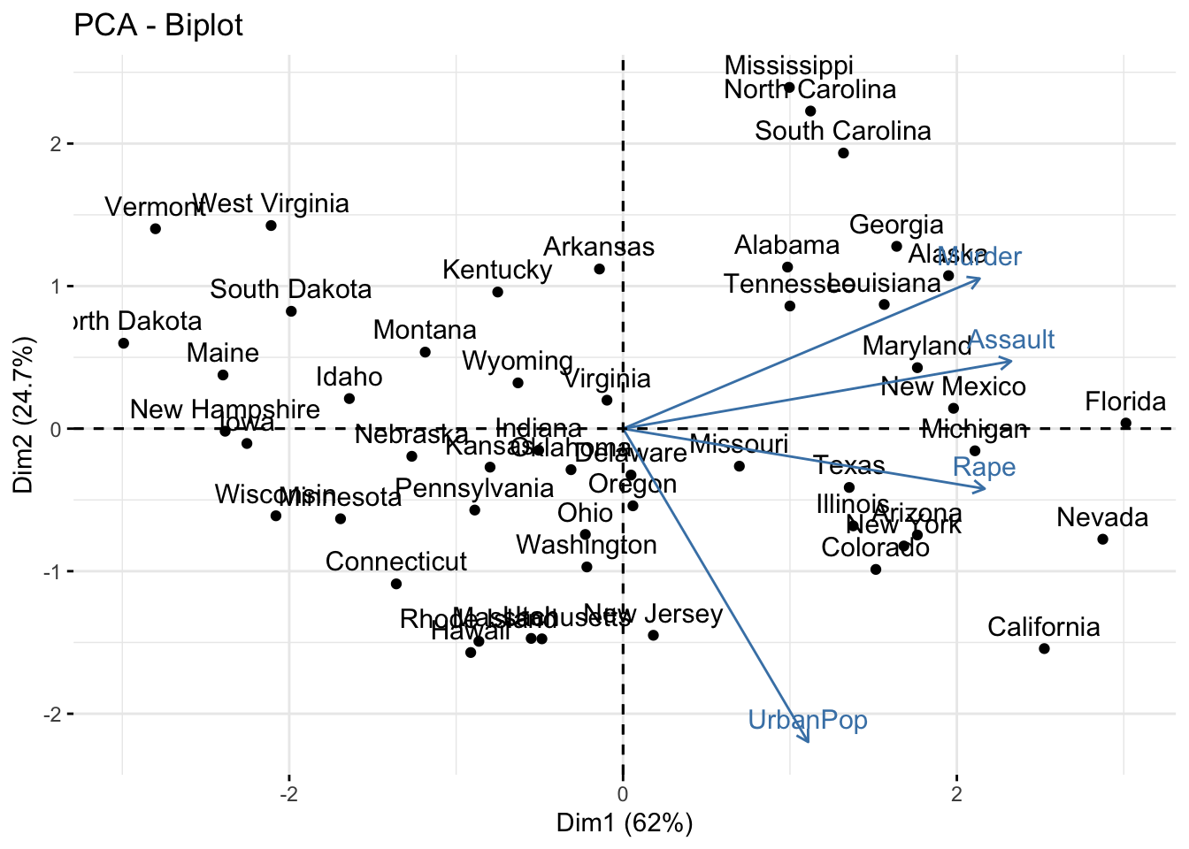
- USArrests data set contains statistics, in arrests per 100,000 residents for assault, murder, and rape in each of the 50 US states in 1973. Also given is the percent of the population living in urban areas.
USArrests %>%str()'data.frame': 50 obs. of 4 variables:
$ Murder : num 13.2 10 8.1 8.8 9 7.9 3.3 5.9 15.4 17.4 ...
$ Assault : int 236 263 294 190 276 204 110 238 335 211 ...
$ UrbanPop: int 58 48 80 50 91 78 77 72 80 60 ...
$ Rape : num 21.2 44.5 31 19.5 40.6 38.7 11.1 15.8 31.9 25.8 ...dat<-USArrests %>%mutate(across(where(is.numeric),scale))
dat %>%str()'data.frame': 50 obs. of 4 variables:
$ Murder : num [1:50, 1] 1.2426 0.5079 0.0716 0.2323 0.2783 ...
..- attr(*, "scaled:center")= num 7.79
..- attr(*, "scaled:scale")= num 4.36
$ Assault : num [1:50, 1] 0.783 1.107 1.479 0.231 1.263 ...
..- attr(*, "scaled:center")= num 171
..- attr(*, "scaled:scale")= num 83.3
$ UrbanPop: num [1:50, 1] -0.521 -1.212 0.999 -1.074 1.759 ...
..- attr(*, "scaled:center")= num 65.5
..- attr(*, "scaled:scale")= num 14.5
$ Rape : num [1:50, 1] -0.00342 2.4842 1.04288 -0.18492 2.06782 ...
..- attr(*, "scaled:center")= num 21.2
..- attr(*, "scaled:scale")= num 9.37- Either princomp or prcomp available in base package of R can be used to perform PCA.
res_pca<-princomp(dat,cor = TRUE,scores = TRUE) # our data is already scaled so any of covariance or correlation matrix will yield same result.
summary(res_pca) # to obtain summary results of PCA
Importance of components:
Comp.1 Comp.2 Comp.3 Comp.4
Standard deviation 1.5748783 0.9948694 0.5971291 0.41644938
Proportion of Variance 0.6200604 0.2474413 0.0891408 0.04335752
Cumulative Proportion 0.6200604 0.8675017 0.9566425 1.00000000screeplot(res_pca,type = "line") # for screeplot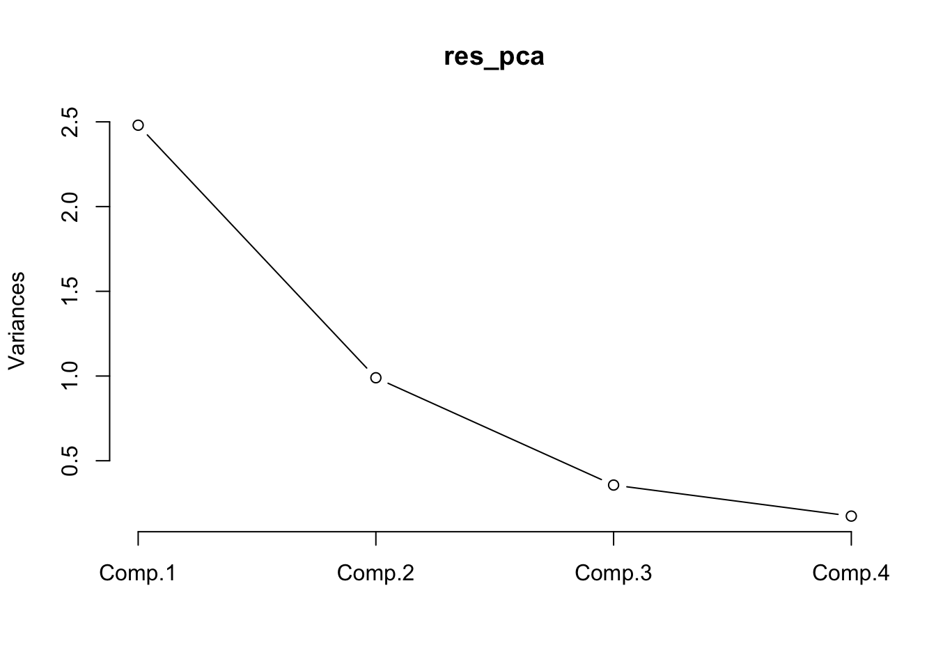
factoextra::fviz_pca_biplot(res_pca) # plotting first 2 PCs